6.5. Cross-validation splitters

As mentioned in the Why cross validation?, cross-validation is a must use technique to evaluate the performance of a model when we don’t have almost infinite data. However, there are several ways to split the data into training and testing sets, and each of them has different properties. In this section we will see why it is important to choose the right cross-validation splitter for your evaluation.

The most important argument is because we want to have an unbiased estimate of the performance of our model, mostly avoiding overestimation. Remember, we are evaluating how well a model will predict unseen data. So if in the future someone uses our model, we want to be sure that it will perform as well as we estimated. If we overestimate the performance, we might be in for a surprise.

Another important argument is that we want to have a good estimate of the variance of our model. This is important because we want to know how much the performance of our model will change if we train it on a different dataset. So which CV splitter should we use? As much as we would like to have an answer to this question, it is impossible for many reasons. According to Bengio and Grandvalet [5], it is simply not possible to have an unbiased estimate of the variance of the generalization error.

We will not repeat what our colleagues from scikit-learn have already explained in their excellent documentation [6]. So we will just add a few words about some topics, assuming you have already read the scikit-learn documentation.

As a rule of thumb, K-fold cross-validation is a good compromise between bias and variance. With K-fold cross-validation, we split the data into K folds, train the model on K-1 folds, and evaluate it on the remaining fold. We repeat this procedure K times, each time using a different fold as the testing set. The final performance is the average of the K performances. The variance of this estimate is lower than the variance of the leave-one-out cross-validation (LOOCV), but higher than the variance of the holdout method. The bias is higher than the bias of LOOCV, but lower than the bias of the holdout method. But these claims must be taken with caution. There has been intense research on this topic, and there are still unconclusive results. While intuition points in one direction, empirical evidence points in other. If you want to know more about this topic, we suggest you start with this thread on Cross Validated [7]. Empirical evidence shows that choosing any K between the extremes [n, 2] is a good compromise between bias and variance. In practice, K=10 is a good choice [8].

Now the fun part begins, which of the many variants of K-fold shall we choose? The answer is: it depends. It depends on the data and the problem you are trying to solve. In this section we will shed some light on two important topics: stratification and grouping.

Stratification

It is a technique used to ensure that the distribution of the target variable is the same in the training and testing sets. This is important because if the distribution of the target variable is different in the training and testing sets, the model will learn a different distribution than the one it will be evaluated on. In a binary classification problem, an extreme example would be if the training set contains only samples of one class, and the testing set contains only samples of the other class. In this case, the model will learn to predict only one class, and it will perform poorly on the testing set. To solve this issue, you can use stratification. That is, you can ensure that the distribution of the target variable is the same in the training and testing sets.

Fortunately, scikit-learn already implements stratification (e.g., stratified K-fold in the sklearn.model_selection.StratifiedKFold). However, this implementation is only valid for discrete target variables. In the case of continuous target variables, julearn comes to rescue you with the ContinuousStratifiedKFold splitter.

The main issue with continuous target variables is that it is not just a simple matter of counting the number of samples of each class. In this case, we need to ensure that the distribution of the target variable is the same in the training and testing sets. This is a more complex problem, and there are several ways to solve it. In julearn, we have implemented two ways of doing this: binning and quantizing.

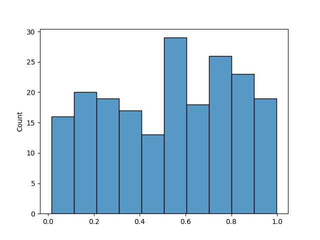
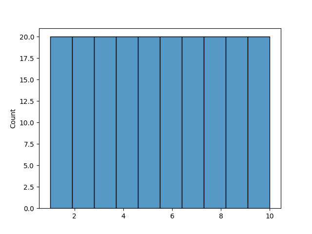
Binning is a technique that consists of dividing the target variable into discrete bins, each of equal size, and then ensuring that the distribution of the target variable is the same in the training and testing sets in terms of samples per bin. Let’s see an example using a uniform distribution, creating 200 samples and 10 bins.

import numpy as np
import matplotlib.pyplot as plt
import seaborn as sns

X = np.random.rand(200, 10)
y = np.random.rand(200)
n_bins = 10

sns.histplot(y, bins=n_bins)

/opt/hostedtoolcache/Python/3.10.14/x64/lib/python3.10/site-packages/seaborn/_oldcore.py:1119: FutureWarning: use_inf_as_na option is deprecated and will be removed in a future version. Convert inf values to NaN before operating instead.
  with pd.option_context('mode.use_inf_as_na', True):

<Axes: ylabel='Count'>

We can see that we have 20 samples per bin. So if we split the data into training and testing sets, we want to ensure that we have the same number of samples per bin in both sets. We can now use the ContinuousStratifiedKFold splitter to generate the indices of the training and testing sets and make a plot to visualize the distribution of the target variable in both sets.

from julearn.model_selection import ContinuousStratifiedKFold

cv = ContinuousStratifiedKFold(
    n_bins=n_bins, n_splits=3, shuffle=True, random_state=42
)

fig, axis = plt.subplots(1, 2, figsize=(20, 4))
train_sets = []
test_sets = []
for train, test in cv.split(X, y):
    train_sets.append(y[train])
    test_sets.append(y[test])

sns.histplot(train_sets, ax=axis[0], bins=n_bins, multiple="dodge", shrink=0.8)
sns.histplot(test_sets, ax=axis[1], bins=n_bins, multiple="dodge", shrink=0.8)

axis[0].set_title("Training sets")
axis[1].set_title("Testing sets")
fig.suptitle(
    "ContinuousStratifiedKFold on uniformly distributed target variable"
)

/opt/hostedtoolcache/Python/3.10.14/x64/lib/python3.10/site-packages/seaborn/_oldcore.py:1119: FutureWarning: use_inf_as_na option is deprecated and will be removed in a future version. Convert inf values to NaN before operating instead.
  with pd.option_context('mode.use_inf_as_na', True):
/opt/hostedtoolcache/Python/3.10.14/x64/lib/python3.10/site-packages/seaborn/_oldcore.py:1119: FutureWarning: use_inf_as_na option is deprecated and will be removed in a future version. Convert inf values to NaN before operating instead.
  with pd.option_context('mode.use_inf_as_na', True):

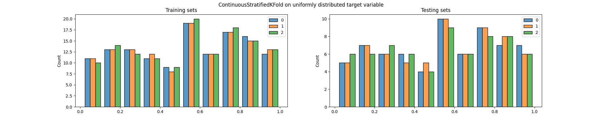
Text(0.5, 0.98, 'ContinuousStratifiedKFold on uniformly distributed target variable')

Now let’s see how K-fold would have split this data.

from sklearn.model_selection import KFold

cv = KFold(n_splits=3, shuffle=True, random_state=42)

fig, axis = plt.subplots(1, 2, figsize=(20, 4))
train_sets = []
test_sets = []
for train, test in cv.split(X, y):
    train_sets.append(y[train])
    test_sets.append(y[test])

sns.histplot(train_sets, ax=axis[0], bins=n_bins, multiple="dodge", shrink=0.8)
sns.histplot(test_sets, ax=axis[1], bins=n_bins, multiple="dodge", shrink=0.8)

axis[0].set_title("Training sets")
axis[1].set_title("Testing sets")
fig.suptitle("K-fold on uniformly distributed target variable")

/opt/hostedtoolcache/Python/3.10.14/x64/lib/python3.10/site-packages/seaborn/_oldcore.py:1119: FutureWarning: use_inf_as_na option is deprecated and will be removed in a future version. Convert inf values to NaN before operating instead.
  with pd.option_context('mode.use_inf_as_na', True):
/opt/hostedtoolcache/Python/3.10.14/x64/lib/python3.10/site-packages/seaborn/_oldcore.py:1119: FutureWarning: use_inf_as_na option is deprecated and will be removed in a future version. Convert inf values to NaN before operating instead.
  with pd.option_context('mode.use_inf_as_na', True):

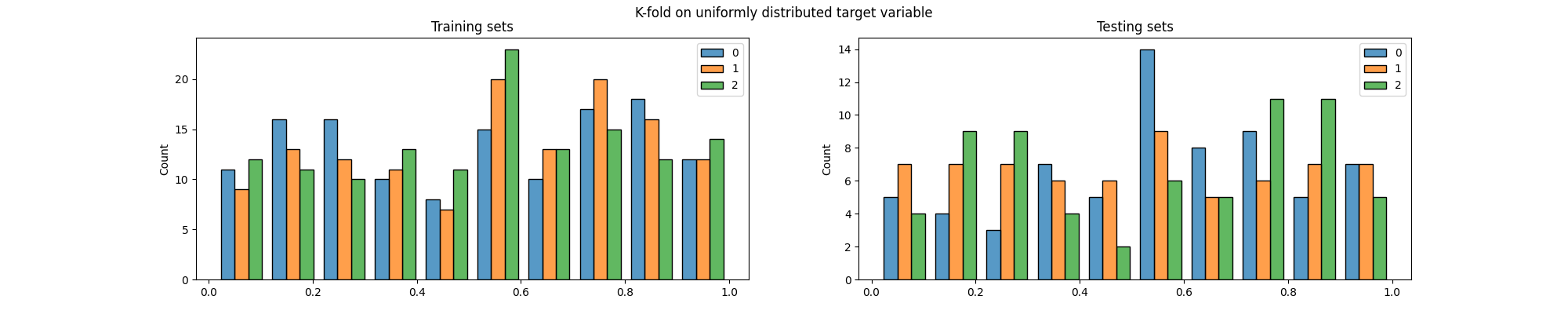
Text(0.5, 0.98, 'K-fold on uniformly distributed target variable')

We can easily see that the distribution of the target variable is not the same in the training and testing sets, particularly across folds.

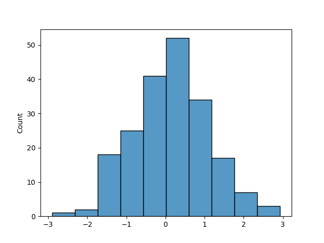
This is a simple example, but it shows the importance of stratification. In practice, the target variable is not uniformly distributed, and the differences between the distributions of the training and testing sets can be much more evident. Let’s take a look at the same analysis but using a Gaussian distribution.

y = np.random.normal(size=200)
sns.histplot(y, bins=n_bins)

/opt/hostedtoolcache/Python/3.10.14/x64/lib/python3.10/site-packages/seaborn/_oldcore.py:1119: FutureWarning: use_inf_as_na option is deprecated and will be removed in a future version. Convert inf values to NaN before operating instead.
  with pd.option_context('mode.use_inf_as_na', True):

<Axes: ylabel='Count'>

cv = ContinuousStratifiedKFold(
    n_bins=n_bins, n_splits=3, shuffle=True, random_state=42
)

fig, axis = plt.subplots(1, 2, figsize=(20, 4))
train_sets = []
test_sets = []
for train, test in cv.split(X, y):
    train_sets.append(y[train])
    test_sets.append(y[test])

sns.histplot(train_sets, ax=axis[0], bins=n_bins, multiple="dodge", shrink=0.8)
sns.histplot(test_sets, ax=axis[1], bins=n_bins, multiple="dodge", shrink=0.8)

axis[0].set_title("Training sets")
axis[1].set_title("Testing sets")
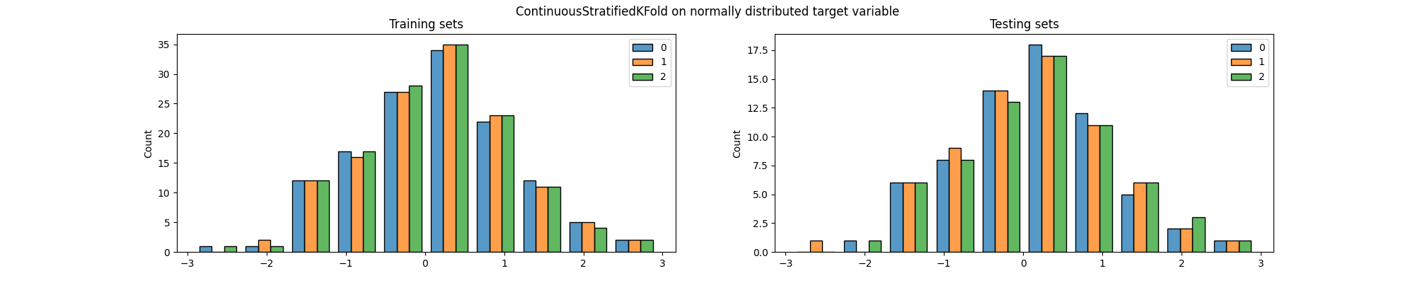
fig.suptitle(
    "ContinuousStratifiedKFold on normally distributed target variable"
)

/opt/hostedtoolcache/Python/3.10.14/x64/lib/python3.10/site-packages/sklearn/model_selection/_split.py:737: UserWarning: The least populated class in y has only 1 members, which is less than n_splits=3.
  warnings.warn(
/opt/hostedtoolcache/Python/3.10.14/x64/lib/python3.10/site-packages/seaborn/_oldcore.py:1119: FutureWarning: use_inf_as_na option is deprecated and will be removed in a future version. Convert inf values to NaN before operating instead.
  with pd.option_context('mode.use_inf_as_na', True):
/opt/hostedtoolcache/Python/3.10.14/x64/lib/python3.10/site-packages/seaborn/_oldcore.py:1119: FutureWarning: use_inf_as_na option is deprecated and will be removed in a future version. Convert inf values to NaN before operating instead.
  with pd.option_context('mode.use_inf_as_na', True):

Text(0.5, 0.98, 'ContinuousStratifiedKFold on normally distributed target variable')

Now lets see how K-fold would have split this data.

cv = KFold(n_splits=3, shuffle=True, random_state=42)

fig, axis = plt.subplots(1, 2, figsize=(20, 4))
train_sets = []
test_sets = []
for train, test in cv.split(X, y):
    train_sets.append(y[train])
    test_sets.append(y[test])

sns.histplot(train_sets, ax=axis[0], bins=n_bins, multiple="dodge", shrink=0.8)
sns.histplot(test_sets, ax=axis[1], bins=n_bins, multiple="dodge", shrink=0.8)

axis[0].set_title("Training sets")
axis[1].set_title("Testing sets")
fig.suptitle("K-fold on normally distributed target variable")

/opt/hostedtoolcache/Python/3.10.14/x64/lib/python3.10/site-packages/seaborn/_oldcore.py:1119: FutureWarning: use_inf_as_na option is deprecated and will be removed in a future version. Convert inf values to NaN before operating instead.
  with pd.option_context('mode.use_inf_as_na', True):
/opt/hostedtoolcache/Python/3.10.14/x64/lib/python3.10/site-packages/seaborn/_oldcore.py:1119: FutureWarning: use_inf_as_na option is deprecated and will be removed in a future version. Convert inf values to NaN before operating instead.
  with pd.option_context('mode.use_inf_as_na', True):

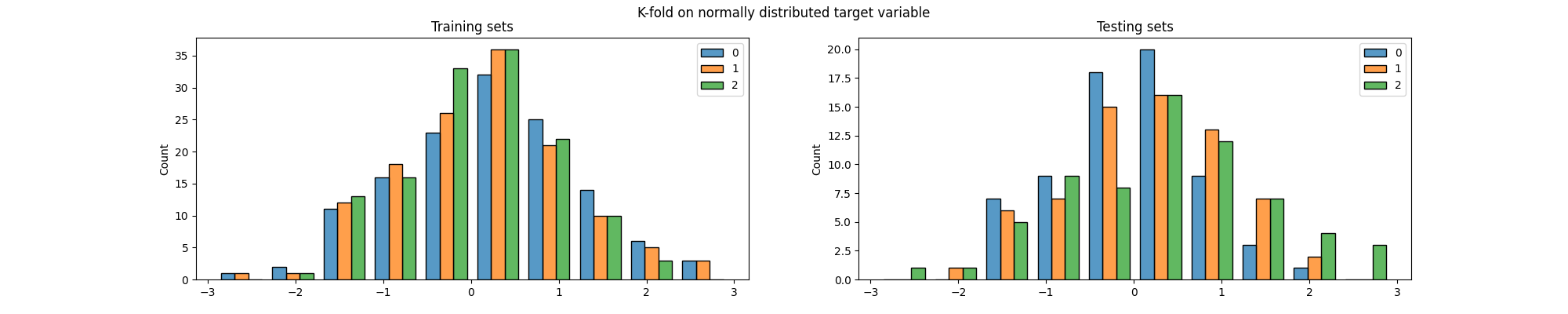
Text(0.5, 0.98, 'K-fold on normally distributed target variable')

Again, we can see that the distribution of the target variable is not the same in the training and testing sets, particularly across folds. But most importantly, both methods generated splits in which some of the classes are (almost) not present in the testing set. This is a problem because it means that the model will not be evaluated on some of the classes, which can lead to biased results.

To this matter, we have implemented a different way of discretizing the target variable. Instead of fixing the size of the bins, we can split the data into bins with the same number of samples. This is called quantizing. Let’s see how this works on the same data.

bins = np.quantile(y, np.linspace(0, 1, n_bins + 1))
discrete_y = np.digitize(y, bins=bins[:-1])
sns.histplot(discrete_y, bins=n_bins)

/opt/hostedtoolcache/Python/3.10.14/x64/lib/python3.10/site-packages/seaborn/_oldcore.py:1119: FutureWarning: use_inf_as_na option is deprecated and will be removed in a future version. Convert inf values to NaN before operating instead.
  with pd.option_context('mode.use_inf_as_na', True):

<Axes: ylabel='Count'>

In this case, each quantile of the target variable is equally represented in each “bin”. To use this approach, we can simply set method="quantile" in the ContinuousStratifiedKFold.

cv = ContinuousStratifiedKFold(
    n_bins=n_bins, method="quantile", n_splits=3, shuffle=True, random_state=42
)

fig, axis = plt.subplots(1, 2, figsize=(20, 4))
train_sets = []
test_sets = []
for train, test in cv.split(X, y):
    train_sets.append(y[train])
    test_sets.append(y[test])

sns.kdeplot(train_sets, ax=axis[0], multiple="layer")
sns.kdeplot(test_sets, ax=axis[1], multiple="layer")

[axis[0].axvline(x, color="k", alpha=0.7, linestyle="--") for x in bins]
[axis[1].axvline(x, color="k", alpha=0.7, linestyle="--") for x in bins]
axis[0].set_title("Training sets")
axis[1].set_title("Testing sets")
fig.suptitle(
    "ContinuousStratifiedKFold (quantile) on normally distributed target variable"
)

/opt/hostedtoolcache/Python/3.10.14/x64/lib/python3.10/site-packages/seaborn/_oldcore.py:1119: FutureWarning: use_inf_as_na option is deprecated and will be removed in a future version. Convert inf values to NaN before operating instead.
  with pd.option_context('mode.use_inf_as_na', True):
/opt/hostedtoolcache/Python/3.10.14/x64/lib/python3.10/site-packages/seaborn/_oldcore.py:1119: FutureWarning: use_inf_as_na option is deprecated and will be removed in a future version. Convert inf values to NaN before operating instead.
  with pd.option_context('mode.use_inf_as_na', True):

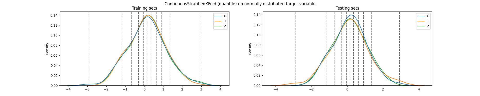
Text(0.5, 0.98, 'ContinuousStratifiedKFold (quantile) on normally distributed target variable')

We can see that the distribution of the target variable is still the same in the training and testing sets, particularly across folds. And most importantly, due to how the bins are defined (dashed lines), each quantile is now equally represented in each fold.

Note

julearn provides RepeatedContinuousStratifiedKFold as the repeated version of ContinuousStratifiedKFold.

Grouping

Another important aspect of cross-validation is grouping. In some cases, we might want to split the data in a way that ensures that samples from the same group are not present in both the training and testing sets. This is particularly important when the data is not independent and identically distributed (i.i.d.). For example, in a study where the same subject is measured multiple times, we might want to ensure that the model is not evaluated on data from the same subject that was used to train it.

To this matter, julearn provides ContinuousStratifiedGroupKFold, which provides support for a grouping variable and RepeatedContinuousStratifiedGroupKFold as the repeated version of it.

References:

[5]

Bengio and Grandvalet, “No Unbiased Estimator of the Variance of K-Fold Cross-Validation” , JMLR, Volume 5, 1 December 2004, pages 1089-1105.

[6]

“Model selection: choosing estimators and their parameters” , scikit-learn documentation.

[7]

https://stats.stackexchange.com/questions/61783/ bias-and-variance-in-leave-one-out-vs-k-fold-cross-validation.

[8]

Kohavi, “A study of cross-validation and bootstrap for accuracy estimation and model selection” , IJCAI’95, pages 1137-1145.