Note
Go to the end to download the full example code.
Regression Analysis
This example uses the diabetes data from sklearn datasets and performs
a regression analysis using a Ridge Regression model.
# Authors: Shammi More <s.more@fz-juelich.de>
#          Federico Raimondo <f.raimondo@fz-juelich.de>
# License: AGPL

import pandas as pd
import seaborn as sns
import numpy as np
import matplotlib.pyplot as plt
from sklearn.datasets import load_diabetes
from sklearn.metrics import mean_absolute_error
from sklearn.model_selection import train_test_split

from julearn import run_cross_validation
from julearn.utils import configure_logging
Set the logging level to info to see extra information.
configure_logging(level="INFO")
2026-06-02 08:30:16,638 - julearn - INFO - ===== Lib Versions =====
2026-06-02 08:30:16,638 - julearn - INFO - numpy: 2.4.6
2026-06-02 08:30:16,638 - julearn - INFO - scipy: 1.17.1
2026-06-02 08:30:16,638 - julearn - INFO - sklearn: 1.8.0
2026-06-02 08:30:16,639 - julearn - INFO - pandas: 3.0.3
2026-06-02 08:30:16,639 - julearn - INFO - julearn: 0.3.6.dev72
2026-06-02 08:30:16,639 - julearn - INFO - ========================
Load the diabetes data from sklearn as a pandas.DataFrame.
features, target = load_diabetes(return_X_y=True, as_frame=True)
Dataset contains ten variables age, sex, body mass index, average blood pressure, and six blood serum measurements (s1-s6) diabetes patients and a quantitative measure of disease progression one year after baseline which is the target we are interested in predicting.
print("Features: \n", features.head())
print("Target: \n", target.describe())
Features:
         age       sex       bmi  ...        s4        s5        s6
0  0.038076  0.050680  0.061696  ... -0.002592  0.019907 -0.017646
1 -0.001882 -0.044642 -0.051474  ... -0.039493 -0.068332 -0.092204
2  0.085299  0.050680  0.044451  ... -0.002592  0.002861 -0.025930
3 -0.089063 -0.044642 -0.011595  ...  0.034309  0.022688 -0.009362
4  0.005383 -0.044642 -0.036385  ... -0.002592 -0.031988 -0.046641

[5 rows x 10 columns]
Target:
 count    442.000000
mean     152.133484
std       77.093005
min       25.000000
25%       87.000000
50%      140.500000
75%      211.500000
max      346.000000
Name: target, dtype: float64
Let’s combine features and target together in one dataframe and define X and y
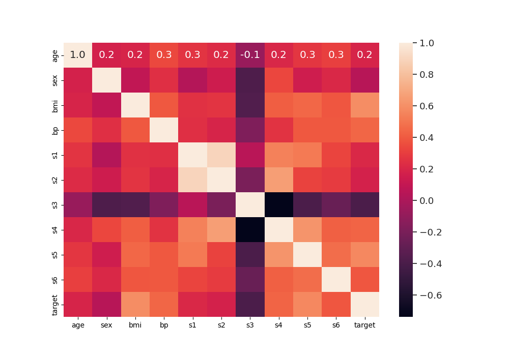
Calculate correlations between the features/variables and plot it as heat map.
corr = data_diabetes.corr()

fig, ax = plt.subplots(1, 1, figsize=(10, 7))
sns.set(font_scale=1.2)
sns.heatmap(
    corr,
    xticklabels=corr.columns,
    yticklabels=corr.columns,
    annot=True,
    fmt="0.1f",
)
<Axes: >
Split the dataset into train and test.
train_diabetes, test_diabetes = train_test_split(data_diabetes, test_size=0.3)
Train a ridge regression model on train dataset and use mean absolute error for scoring.
2026-06-02 08:30:16,840 - julearn - INFO - ==== Input Data ====
2026-06-02 08:30:16,841 - julearn - INFO - Using dataframe as input
2026-06-02 08:30:16,841 - julearn - INFO -      Features: ['age', 'sex', 'bmi', 'bp', 's1', 's2', 's3', 's4', 's5', 's6']
2026-06-02 08:30:16,841 - julearn - INFO -      Target: target
2026-06-02 08:30:16,841 - julearn - INFO -      Expanded features: ['age', 'sex', 'bmi', 'bp', 's1', 's2', 's3', 's4', 's5', 's6']
2026-06-02 08:30:16,841 - julearn - INFO -      X_types:{}
2026-06-02 08:30:16,841 - julearn - WARNING - The following columns are not defined in X_types: ['age', 'sex', 'bmi', 'bp', 's1', 's2', 's3', 's4', 's5', 's6']. They will be treated as continuous.
/tmp/tmpe_uj5qr7/julearn/prepare.py:609: RuntimeWarning: The following columns are not defined in X_types: ['age', 'sex', 'bmi', 'bp', 's1', 's2', 's3', 's4', 's5', 's6']. They will be treated as continuous.
  warn_with_log(
2026-06-02 08:30:16,842 - julearn - INFO - ====================
2026-06-02 08:30:16,843 - julearn - INFO -
2026-06-02 08:30:16,843 - julearn - INFO - Adding step zscore that applies to ColumnTypes<types={'continuous'}; pattern=(?:__:type:__continuous)>
2026-06-02 08:30:16,843 - julearn - INFO - Step added
2026-06-02 08:30:16,843 - julearn - INFO - Adding step ridge that applies to ColumnTypes<types={'continuous'}; pattern=(?:__:type:__continuous)>
2026-06-02 08:30:16,843 - julearn - INFO - Step added
2026-06-02 08:30:16,844 - julearn - INFO - = Model Parameters =
2026-06-02 08:30:16,844 - julearn - INFO - ====================
2026-06-02 08:30:16,844 - julearn - INFO -
2026-06-02 08:30:16,844 - julearn - INFO - = Data Information =
2026-06-02 08:30:16,844 - julearn - INFO -      Problem type: regression
2026-06-02 08:30:16,844 - julearn - INFO -      Number of samples: 309
2026-06-02 08:30:16,844 - julearn - INFO -      Number of features: 10
2026-06-02 08:30:16,844 - julearn - INFO - ====================
2026-06-02 08:30:16,844 - julearn - INFO -
2026-06-02 08:30:16,844 - julearn - INFO -      Target type: float64
2026-06-02 08:30:16,845 - julearn - INFO - Using outer CV scheme KFold(n_splits=5, random_state=None, shuffle=False) (incl. final model)
The scores dataframe has all the values for each CV split.
Mean value of mean absolute error across CV
print(scores["test_score"].mean() * -1)
45.444084441470615
Now we can get the MAE fold and repetition:
df_mae = scores.set_index(["repeat", "fold"])["test_score"].unstack() * -1
df_mae.index.name = "Repeats"
df_mae.columns.name = "K-fold splits"

df_mae
Plot heatmap of mean absolute error (MAE) over all repeats and CV splits.
fig, ax = plt.subplots(1, 1, figsize=(10, 7))
sns.heatmap(df_mae, cmap="YlGnBu")
plt.title("Cross-validation MAE")
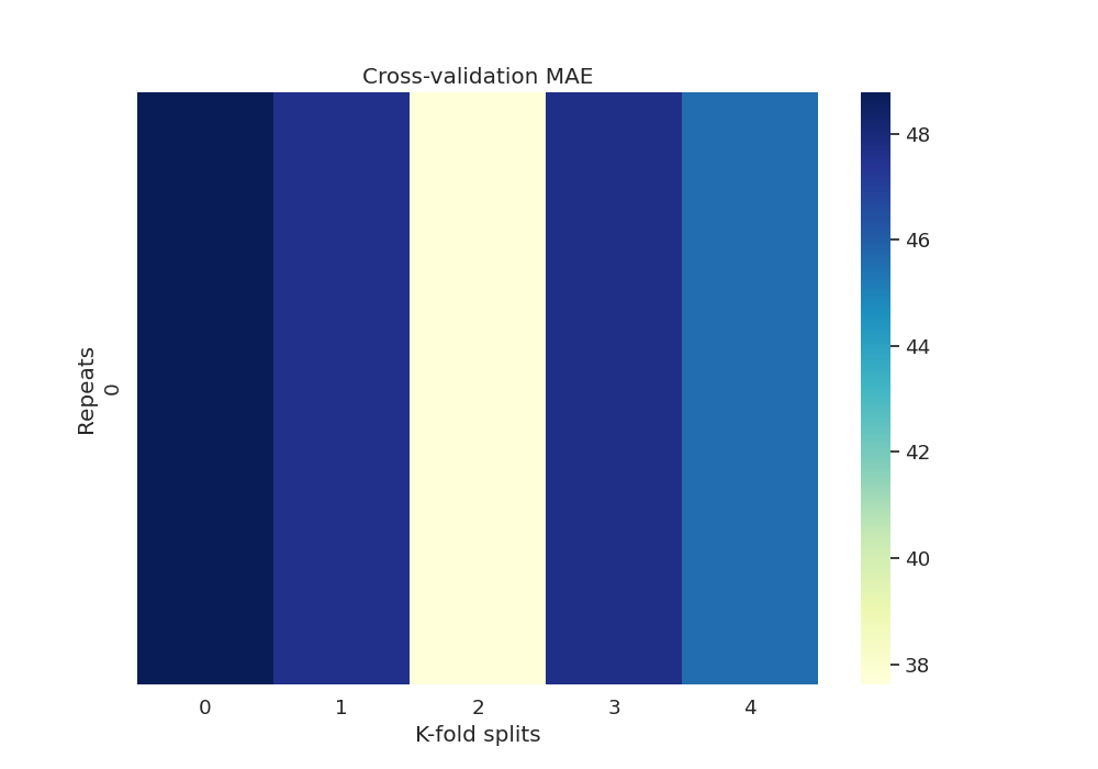
Text(0.5, 1.0, 'Cross-validation MAE')
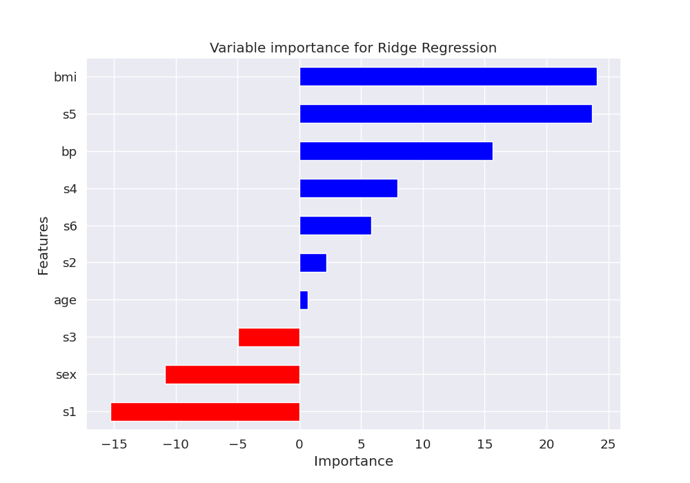
Let’s plot the feature importance using the coefficients of the trained model.
features = pd.DataFrame({"Features": X, "importance": model["ridge"].coef_})
features.sort_values(by=["importance"], ascending=True, inplace=True)
features["positive"] = features["importance"] > 0

fig, ax = plt.subplots(1, 1, figsize=(10, 7))
features.set_index("Features", inplace=True)
features.importance.plot(
    kind="barh", color=features.positive.map({True: "blue", False: "red"})
)
ax.set(xlabel="Importance", title="Variable importance for Ridge Regression")
[Text(0.5, 40.249999999999986, 'Importance'), Text(0.5, 1.0, 'Variable importance for Ridge Regression')]
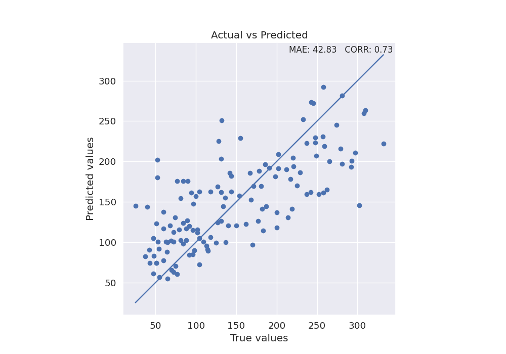
Use the final model to make predictions on test data and plot scatterplot of true values vs predicted values.
y_true = test_diabetes[y]
y_pred = model.predict(test_diabetes[X])
mae = format(mean_absolute_error(y_true, y_pred), ".2f")
corr = format(np.corrcoef(y_pred, y_true)[1, 0], ".2f")

fig, ax = plt.subplots(1, 1, figsize=(10, 7))
sns.set_style("darkgrid")
plt.scatter(y_true, y_pred)
plt.plot(y_true, y_true)
xmin, xmax = ax.get_xlim()
ymin, ymax = ax.get_ylim()
text = "MAE: " + str(mae) + "   CORR: " + str(corr)
ax.set(xlabel="True values", ylabel="Predicted values")
plt.title("Actual vs Predicted")
plt.text(
    xmax - 0.01 * xmax,
    ymax - 0.01 * ymax,
    text,
    verticalalignment="top",
    horizontalalignment="right",
    fontsize=12,
)
plt.axis("scaled")
(np.float64(9.649999999999999), np.float64(347.35), np.float64(9.649999999999999), np.float64(347.35))
Total running time of the script: (0 minutes 0.533 seconds)