Note
Go to the end to download the full example code.
Regression Analysis
This example uses the diabetes data from sklearn datasets and performs
a regression analysis using a Ridge Regression model. We’ll use the
julearn.PipelineCreator to create a pipeline with two different PCA steps and
reduce the dimensionality of the data, each one computed on a different
subset of features.
# Authors: Georgios Antonopoulos <g.antonopoulos@fz-juelich.de>
#          Kaustubh R. Patil <k.patil@fz-juelich.de>
#          Shammi More <s.more@fz-juelich.de>
#          Federico Raimondo <f.raimondo@fz-juelich.de>
# License: AGPL

import pandas as pd
import seaborn as sns
import numpy as np
import matplotlib.pyplot as plt
from sklearn.datasets import load_diabetes
from sklearn.metrics import mean_absolute_error
from sklearn.model_selection import train_test_split

from julearn import run_cross_validation
from julearn.utils import configure_logging
from julearn.pipeline import PipelineCreator
from julearn.inspect import preprocess
Set the logging level to info to see extra information.
configure_logging(level="INFO")
2026-06-02 08:30:40,313 - julearn - INFO - ===== Lib Versions =====
2026-06-02 08:30:40,314 - julearn - INFO - numpy: 2.4.6
2026-06-02 08:30:40,314 - julearn - INFO - scipy: 1.17.1
2026-06-02 08:30:40,314 - julearn - INFO - sklearn: 1.8.0
2026-06-02 08:30:40,314 - julearn - INFO - pandas: 3.0.3
2026-06-02 08:30:40,314 - julearn - INFO - julearn: 0.3.6.dev72
2026-06-02 08:30:40,314 - julearn - INFO - ========================
Load the diabetes data from sklearn as a pandas.DataFrame.
features, target = load_diabetes(return_X_y=True, as_frame=True)
Dataset contains ten variables age, sex, body mass index, average blood pressure, and six blood serum measurements (s1-s6) diabetes patients and a quantitative measure of disease progression one year after baseline which is the target we are interested in predicting.
print("Features: \n", features.head())
print("Target: \n", target.describe())
Features:
         age       sex       bmi  ...        s4        s5        s6
0  0.038076  0.050680  0.061696  ... -0.002592  0.019907 -0.017646
1 -0.001882 -0.044642 -0.051474  ... -0.039493 -0.068332 -0.092204
2  0.085299  0.050680  0.044451  ... -0.002592  0.002861 -0.025930
3 -0.089063 -0.044642 -0.011595  ...  0.034309  0.022688 -0.009362
4  0.005383 -0.044642 -0.036385  ... -0.002592 -0.031988 -0.046641

[5 rows x 10 columns]
Target:
 count    442.000000
mean     152.133484
std       77.093005
min       25.000000
25%       87.000000
50%      140.500000
75%      211.500000
max      346.000000
Name: target, dtype: float64
Let’s combine features and target together in one dataframe and define X and y
Assign types to the features and create feature groups for PCA. We will keep 1 component per PCA group.
X_types = {
    "pca1": ["age", "bmi", "bp"],
    "pca2": ["s1", "s2", "s3", "s4", "s5", "s6"],
    "categorical": ["sex"],
}
Create a pipeline to process the data and the fit a model. We must specify
how each X_type will be used. For example if in the last step we do not
specify apply_to=["continuous", "categorical"], then the pipeline will not
know what to do with the categorical features.
creator = PipelineCreator(problem_type="regression")
creator.add("pca", apply_to="pca1", n_components=1, name="pca_feats1")
creator.add("pca", apply_to="pca2", n_components=1, name="pca_feats2")
creator.add("ridge", apply_to=["continuous", "categorical"])
2026-06-02 08:30:40,330 - julearn - INFO - Adding step pca_feats1 that applies to ColumnTypes<types={'pca1'}; pattern=(?:__:type:__pca1)>
2026-06-02 08:30:40,330 - julearn - INFO - Setting hyperparameter n_components = 1
2026-06-02 08:30:40,330 - julearn - INFO - Step added
2026-06-02 08:30:40,331 - julearn - INFO - Adding step pca_feats2 that applies to ColumnTypes<types={'pca2'}; pattern=(?:__:type:__pca2)>
2026-06-02 08:30:40,331 - julearn - INFO - Setting hyperparameter n_components = 1
2026-06-02 08:30:40,331 - julearn - INFO - Step added
2026-06-02 08:30:40,331 - julearn - INFO - Adding step ridge that applies to ColumnTypes<types={'categorical', 'continuous'}; pattern=(?:__:type:__categorical|__:type:__continuous)>
2026-06-02 08:30:40,331 - julearn - INFO - Step added

<julearn.pipeline.pipeline_creator.PipelineCreator object at 0x7f029957e250>
Split the dataset into train and test.
train_diabetes, test_diabetes = train_test_split(data_diabetes, test_size=0.3)
Train a ridge regression model on train dataset and use mean absolute error for scoring.
2026-06-02 08:30:40,333 - julearn - INFO - ==== Input Data ====
2026-06-02 08:30:40,333 - julearn - INFO - Using dataframe as input
2026-06-02 08:30:40,333 - julearn - INFO -      Features: ['age', 'sex', 'bmi', 'bp', 's1', 's2', 's3', 's4', 's5', 's6']
2026-06-02 08:30:40,333 - julearn - INFO -      Target: target
2026-06-02 08:30:40,333 - julearn - INFO -      Expanded features: ['age', 'sex', 'bmi', 'bp', 's1', 's2', 's3', 's4', 's5', 's6']
2026-06-02 08:30:40,334 - julearn - INFO -      X_types:{'pca1': ['age', 'bmi', 'bp'], 'pca2': ['s1', 's2', 's3', 's4', 's5', 's6'], 'categorical': ['sex']}
2026-06-02 08:30:40,335 - julearn - INFO - ====================
2026-06-02 08:30:40,335 - julearn - INFO -
2026-06-02 08:30:40,335 - julearn - INFO - = Model Parameters =
2026-06-02 08:30:40,336 - julearn - INFO - ====================
2026-06-02 08:30:40,336 - julearn - INFO -
2026-06-02 08:30:40,336 - julearn - INFO - = Data Information =
2026-06-02 08:30:40,336 - julearn - INFO -      Problem type: regression
2026-06-02 08:30:40,336 - julearn - INFO -      Number of samples: 309
2026-06-02 08:30:40,336 - julearn - INFO -      Number of features: 10
2026-06-02 08:30:40,336 - julearn - INFO - ====================
2026-06-02 08:30:40,336 - julearn - INFO -
2026-06-02 08:30:40,336 - julearn - INFO -      Target type: float64
2026-06-02 08:30:40,336 - julearn - INFO - Using outer CV scheme KFold(n_splits=5, random_state=None, shuffle=False) (incl. final model)
The scores dataframe has all the values for each CV split.
print(scores.head())
   fit_time  score_time  ...  fold                          cv_mdsum
0  0.014539    0.006609  ...     0  b10eef89b4192178d482d7a1587a248a
1  0.014362    0.006688  ...     1  b10eef89b4192178d482d7a1587a248a
2  0.014797    0.006634  ...     2  b10eef89b4192178d482d7a1587a248a
3  0.014224    0.006632  ...     3  b10eef89b4192178d482d7a1587a248a
4  0.014547    0.006708  ...     4  b10eef89b4192178d482d7a1587a248a

[5 rows x 8 columns]
Mean value of mean absolute error across CV.
print(scores["test_score"].mean())
0.3107976743678922
Let’s see how the data looks like after preprocessing. We will process the data until the first PCA step. We should get the first PCA component for [“age”, “bmi”, “bp”] and leave other features untouched.
data_processed1 = preprocess(model, X, data=train_diabetes, until="pca_feats1")
print("Data after preprocessing until PCA step 1")
data_processed1.head()
Data after preprocessing until PCA step 1
We will process the data until the second PCA step. We should now also get one PCA component for [“s1”, “s2”, “s3”, “s4”, “s5”, “s6”].
data_processed2 = preprocess(model, X, data=train_diabetes, until="pca_feats2")
print("Data after preprocessing until PCA step 2")
data_processed2.head()
Data after preprocessing until PCA step 2
Now we can get the MAE fold and repetition:
df_mae = scores.set_index(["repeat", "fold"])["test_score"].unstack() * -1
df_mae.index.name = "Repeats"
df_mae.columns.name = "K-fold splits"

print(df_mae)
K-fold splits         0         1         2         3         4
Repeats
0             -0.341472 -0.348168 -0.269257 -0.286067 -0.309025
Plot heatmap of mean absolute error (MAE) over all repeats and CV splits.
fig, ax = plt.subplots(1, 1, figsize=(10, 7))
sns.heatmap(df_mae, cmap="YlGnBu")
plt.title("Cross-validation MAE")
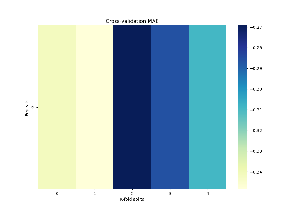
Text(0.5, 1.0, 'Cross-validation MAE')
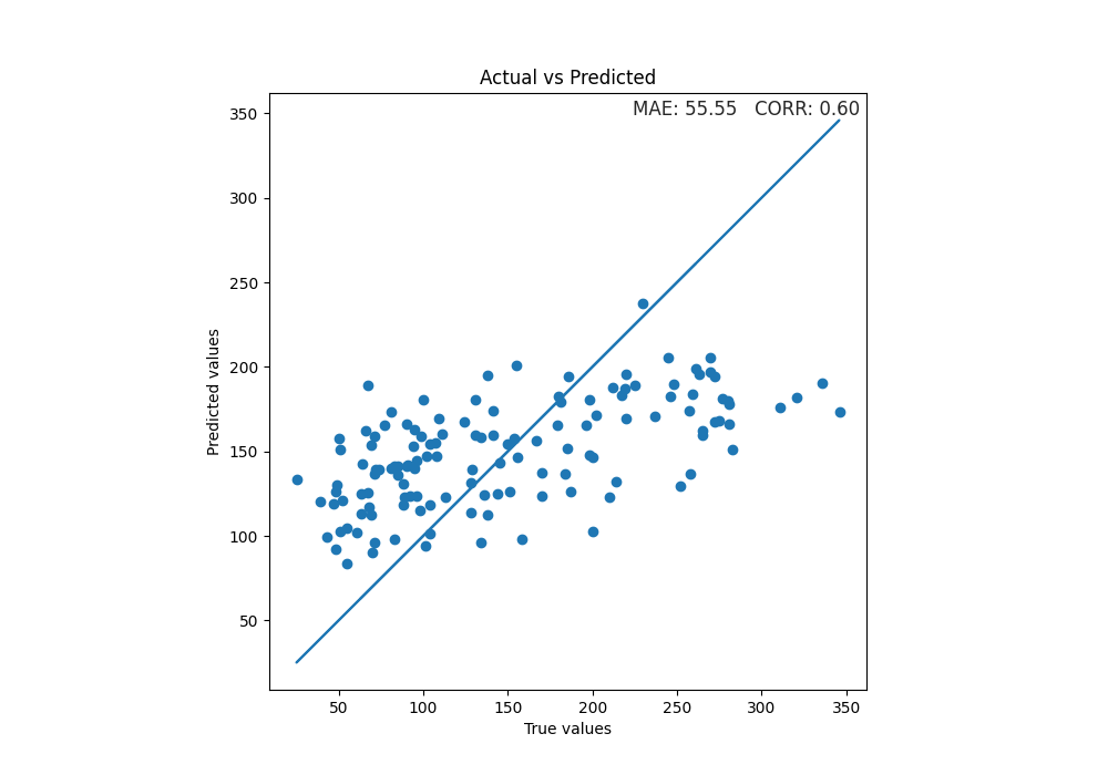
Use the final model to make predictions on test data and plot scatterplot of true values vs predicted values.
y_true = test_diabetes[y]
y_pred = model.predict(test_diabetes[X])
mae = format(mean_absolute_error(y_true, y_pred), ".2f")
corr = format(np.corrcoef(y_pred, y_true)[1, 0], ".2f")

fig, ax = plt.subplots(1, 1, figsize=(10, 7))
sns.set_style("darkgrid")
plt.scatter(y_true, y_pred)
plt.plot(y_true, y_true)
xmin, xmax = ax.get_xlim()
ymin, ymax = ax.get_ylim()
text = "MAE: " + str(mae) + "   CORR: " + str(corr)
ax.set(xlabel="True values", ylabel="Predicted values")
plt.title("Actual vs Predicted")
plt.text(
    xmax - 0.01 * xmax,
    ymax - 0.01 * ymax,
    text,
    verticalalignment="top",
    horizontalalignment="right",
    fontsize=12,
)
plt.axis("scaled")
(np.float64(8.95), np.float64(362.05), np.float64(8.95), np.float64(362.05))
Total running time of the script: (0 minutes 0.366 seconds)