Note
Go to the end to download the full example code.
Confound Removal (model comparison)
This example uses the iris dataset, performs simple binary classification
with and without confound removal using a Random Forest classifier.
# Authors: Shammi More <s.more@fz-juelich.de>
#          Federico Raimondo <f.raimondo@fz-juelich.de>
#          Leonard Sasse <l.sasse@fz-juelich.de>
# License: AGPL

import matplotlib.pyplot as plt
import pandas as pd
import seaborn as sns
from seaborn import load_dataset

from julearn import run_cross_validation
from julearn.model_selection import StratifiedBootstrap
from julearn.pipeline import PipelineCreator
from julearn.utils import configure_logging
Set the logging level to info to see extra information.
configure_logging(level="INFO")
2026-07-21 10:58:45,754 - julearn - INFO - ===== Lib Versions =====
2026-07-21 10:58:45,754 - julearn - INFO - numpy: 2.5.1
2026-07-21 10:58:45,754 - julearn - INFO - scipy: 1.18.0
2026-07-21 10:58:45,755 - julearn - INFO - sklearn: 1.8.0
2026-07-21 10:58:45,755 - julearn - INFO - pandas: 3.0.3
2026-07-21 10:58:45,755 - julearn - INFO - julearn: 0.3.6.dev75
2026-07-21 10:58:45,755 - julearn - INFO - ========================
Load the iris data from seaborn.
df_iris = load_dataset("iris")
The dataset has three kind of species. We will keep two to perform a binary classification.
As features, we will use the sepal length, width and petal length and use petal width as confound.
Doing hypothesis testing in ML is not that simple. If we were to use classical frequentist statistics, we have the problem that using cross validation, the samples are not independent and the population (train + test) is always the same.
If we want to compare two models, an alternative is to contrast, for each fold, the performance gap between the models. If we combine that approach with bootstrapping, we can then compare the confidence intervals of the difference. If the 95% CI is above 0 (or below), we can claim that the models are different with p < 0.05.
Let’s use a bootstrap CV. In the interest of time we do 20 iterations, change the number of bootstrap iterations to at least 2000 for a valid test.
n_bootstrap = 20
n_elements = len(df_iris)
cv = StratifiedBootstrap(n_splits=n_bootstrap, random_state=42)
First, we will train a model without performing confound removal on features. Note: confounds by default.
2026-07-21 10:58:45,758 - julearn - INFO - Setting random seed to 200
2026-07-21 10:58:45,758 - julearn - INFO - ==== Input Data ====
2026-07-21 10:58:45,758 - julearn - INFO - Using dataframe as input
2026-07-21 10:58:45,758 - julearn - INFO -      Features: ['sepal_length', 'sepal_width', 'petal_length']
2026-07-21 10:58:45,758 - julearn - INFO -      Target: species
2026-07-21 10:58:45,759 - julearn - INFO -      Expanded features: ['sepal_length', 'sepal_width', 'petal_length']
2026-07-21 10:58:45,759 - julearn - INFO -      X_types:{}
2026-07-21 10:58:45,759 - julearn - WARNING - The following columns are not defined in X_types: ['sepal_length', 'sepal_width', 'petal_length']. They will be treated as continuous.
/tmp/tmpp8_t5ngz/julearn/prepare.py:609: RuntimeWarning: The following columns are not defined in X_types: ['sepal_length', 'sepal_width', 'petal_length']. They will be treated as continuous.
  warn_with_log(
2026-07-21 10:58:45,760 - julearn - INFO - ====================
2026-07-21 10:58:45,760 - julearn - INFO -
2026-07-21 10:58:45,760 - julearn - INFO - Adding step zscore that applies to ColumnTypes<types={'continuous'}; pattern=(?:__:type:__continuous)>
2026-07-21 10:58:45,761 - julearn - INFO - Step added
2026-07-21 10:58:45,761 - julearn - INFO - Adding step rf that applies to ColumnTypes<types={'continuous'}; pattern=(?:__:type:__continuous)>
2026-07-21 10:58:45,761 - julearn - INFO - Step added
2026-07-21 10:58:45,761 - julearn - INFO - = Model Parameters =
2026-07-21 10:58:45,762 - julearn - INFO - ====================
2026-07-21 10:58:45,762 - julearn - INFO -
2026-07-21 10:58:45,762 - julearn - INFO - = Data Information =
2026-07-21 10:58:45,762 - julearn - INFO -      Problem type: classification
2026-07-21 10:58:45,762 - julearn - INFO -      Number of samples: 100
2026-07-21 10:58:45,762 - julearn - INFO -      Number of features: 3
2026-07-21 10:58:45,763 - julearn - INFO - ====================
2026-07-21 10:58:45,763 - julearn - INFO -
2026-07-21 10:58:45,763 - julearn - INFO -      Number of classes: 2
2026-07-21 10:58:45,763 - julearn - INFO -      Target type: str
2026-07-21 10:58:45,764 - julearn - INFO -      Class distributions: species
versicolor    50
virginica     50
Name: count, dtype: int64
2026-07-21 10:58:45,765 - julearn - INFO - Using outer CV scheme StratifiedBootstrap(n_splits=20, random_state=42)
2026-07-21 10:58:45,765 - julearn - WARNING - The kind of values in y (str) is not suitable for a classification. Values should be numeric.
/tmp/tmpp8_t5ngz/julearn/prepare.py:422: RuntimeWarning: The kind of values in y (str) is not suitable for a classification. Values should be numeric.
  warn_with_log(
2026-07-21 10:58:45,765 - julearn - INFO - Binary classification problem detected.
Next, we train a model after performing confound removal on the features. Note: we initialize the CV again to use the same folds as before.
cv = StratifiedBootstrap(n_splits=n_bootstrap, random_state=42)

# In order to tell ``run_cross_validation`` which columns are confounds,
# and which columns are features, we have to define the X_types:
X_types = {"features": X, "confound": confounds}
We can now define a pipeline creator and add a confound removal step. The pipeline creator should apply all the steps, by default, to the features type.
The first step will zscore both features and confounds.
The second step will remove the confounds (type “confound”) from the “features”.
Finally, a random forest will be trained.
Given the default apply_to in the pipeline creator,
the random forest will only be trained using “features”.
creator = PipelineCreator(problem_type="classification", apply_to="features")
creator.add("zscore", apply_to=["features", "confound"])
creator.add("confound_removal", apply_to="features", confounds="confound")
creator.add("rf")

scores_cr = run_cross_validation(
    X=X + confounds,
    y=y,
    data=df_iris,
    model=creator,
    cv=cv,
    X_types=X_types,
    scoring=["accuracy", "roc_auc"],
    return_estimator="cv",
    seed=200,
)
2026-07-21 10:58:48,586 - julearn - INFO - Adding step zscore that applies to ColumnTypes<types={'confound', 'features'}; pattern=(?:__:type:__confound|__:type:__features)>
2026-07-21 10:58:48,587 - julearn - INFO - Step added
2026-07-21 10:58:48,587 - julearn - INFO - Adding step confound_removal that applies to ColumnTypes<types={'features'}; pattern=(?:__:type:__features)>
2026-07-21 10:58:48,587 - julearn - INFO - Setting hyperparameter confounds = confound
2026-07-21 10:58:48,588 - julearn - INFO - Step added
2026-07-21 10:58:48,588 - julearn - INFO - Adding step rf that applies to ColumnTypes<types={'features'}; pattern=(?:__:type:__features)>
2026-07-21 10:58:48,588 - julearn - INFO - Step added
2026-07-21 10:58:48,588 - julearn - INFO - Setting random seed to 200
2026-07-21 10:58:48,588 - julearn - INFO - ==== Input Data ====
2026-07-21 10:58:48,588 - julearn - INFO - Using dataframe as input
2026-07-21 10:58:48,589 - julearn - INFO -      Features: ['sepal_length', 'sepal_width', 'petal_length', 'petal_width']
2026-07-21 10:58:48,589 - julearn - INFO -      Target: species
2026-07-21 10:58:48,589 - julearn - INFO -      Expanded features: ['sepal_length', 'sepal_width', 'petal_length', 'petal_width']
2026-07-21 10:58:48,589 - julearn - INFO -      X_types:{'features': ['sepal_length', 'sepal_width', 'petal_length'], 'confound': ['petal_width']}
2026-07-21 10:58:48,590 - julearn - INFO - ====================
2026-07-21 10:58:48,590 - julearn - INFO -
2026-07-21 10:58:48,591 - julearn - INFO - = Model Parameters =
2026-07-21 10:58:48,591 - julearn - INFO - ====================
2026-07-21 10:58:48,591 - julearn - INFO -
2026-07-21 10:58:48,591 - julearn - INFO - = Data Information =
2026-07-21 10:58:48,591 - julearn - INFO -      Problem type: classification
2026-07-21 10:58:48,592 - julearn - INFO -      Number of samples: 100
2026-07-21 10:58:48,592 - julearn - INFO -      Number of features: 4
2026-07-21 10:58:48,592 - julearn - INFO - ====================
2026-07-21 10:58:48,592 - julearn - INFO -
2026-07-21 10:58:48,592 - julearn - INFO -      Number of classes: 2
2026-07-21 10:58:48,592 - julearn - INFO -      Target type: str
2026-07-21 10:58:48,593 - julearn - INFO -      Class distributions: species
versicolor    50
virginica     50
Name: count, dtype: int64
2026-07-21 10:58:48,594 - julearn - INFO - Using outer CV scheme StratifiedBootstrap(n_splits=20, random_state=42)
2026-07-21 10:58:48,594 - julearn - WARNING - The kind of values in y (str) is not suitable for a classification. Values should be numeric.
/tmp/tmpp8_t5ngz/julearn/prepare.py:422: RuntimeWarning: The kind of values in y (str) is not suitable for a classification. Values should be numeric.
  warn_with_log(
2026-07-21 10:58:48,595 - julearn - INFO - Binary classification problem detected.
Now we can compare the accuracies. We can combine the two outputs as
pandas.DataFrame.
scores_ncr["confounds"] = "Not Removed"
scores_cr["confounds"] = "Removed"
Now we convert the metrics to a column for easier seaborn plotting (convert to long format).
index = ["fold", "confounds"]
scorings = ["test_accuracy", "test_roc_auc"]

df_ncr_metrics = scores_ncr.set_index(index)[scorings].stack()
df_ncr_metrics.index.names = ["fold", "confounds", "metric"]
df_ncr_metrics.name = "value"

df_cr_metrics = scores_cr.set_index(index)[scorings].stack()
df_cr_metrics.index.names = ["fold", "confounds", "metric"]
df_cr_metrics.name = "value"

df_metrics = pd.concat((df_ncr_metrics, df_cr_metrics))

df_metrics = df_metrics.reset_index()
df_metrics.head()
And finally plot the results.
sns.catplot(
    x="confounds", y="value", col="metric", data=df_metrics, kind="swarm"
)
plt.tight_layout()
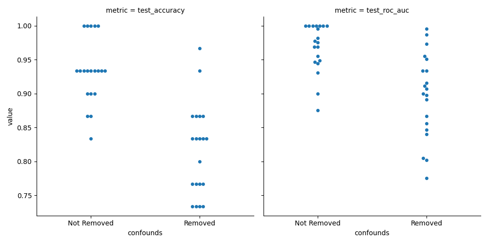
While this plot allows us to see the mean performance values and compare them, these samples are paired. In order to see if there is a systematic difference, we need to check the distribution of differences between the the models.
First, we remove the column “confounds” from the index and make the difference between the metrics.
df_cr_metrics = df_cr_metrics.reset_index().set_index(["fold", "metric"])
df_ncr_metrics = df_ncr_metrics.reset_index().set_index(["fold", "metric"])

df_diff_metrics = df_ncr_metrics["value"] - df_cr_metrics["value"]
df_diff_metrics = df_diff_metrics.reset_index()
Now we can finally plot the difference, setting the whiskers of the box plot at 2.5 and 97.5 to see the 95% CI.
sns.boxplot(
    x="metric", y="value", data=df_diff_metrics.reset_index(), whis=[2.5, 97.5]
)
plt.axhline(0, color="k", ls=":")
plt.tight_layout()
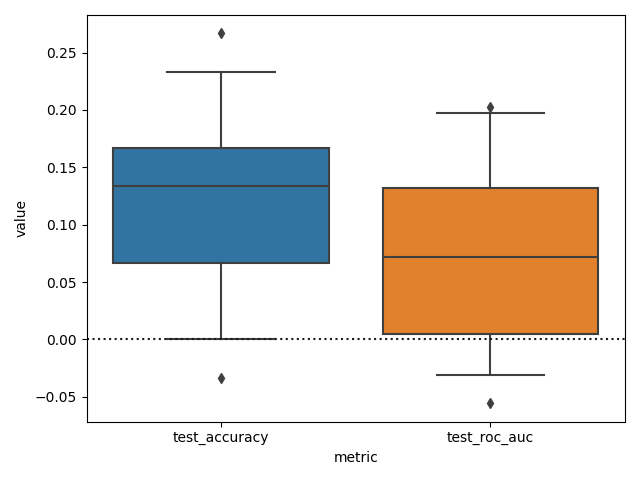
We can see that while it seems that the accuracy and ROC AUC scores are higher when confounds are not removed. We can not really claim (using this test), that the models are different in terms of these metrics.
Maybe the percentiles will be more accuracy with the proper amount of bootstrap iterations?
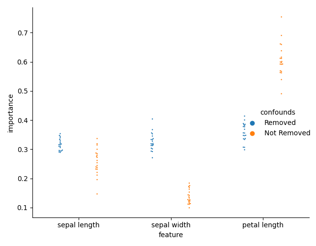
But the main point of confound removal is for interpretability. Let’s see if there is a change in the feature importances.
First, we need to collect the feature importances for each model, for each fold.
ncr_fi = []
for i_fold, estimator in enumerate(scores_ncr["estimator"]):
    this_importances = pd.DataFrame(
        {
            "feature": [x.replace("_", " ") for x in X],
            "importance": estimator["rf"].feature_importances_,
            "confounds": "Not Removed",
            "fold": i_fold,
        }
    )
    ncr_fi.append(this_importances)
ncr_fi = pd.concat(ncr_fi)

cr_fi = []
for i_fold, estimator in enumerate(scores_cr["estimator"]):
    this_importances = pd.DataFrame(
        {
            "feature": [x.replace("_", " ") for x in X],
            "importance": estimator["rf"].model.feature_importances_,
            "confounds": "Removed",
            "fold": i_fold,
        }
    )
    cr_fi.append(this_importances)
cr_fi = pd.concat(cr_fi)

feature_importance = pd.concat([cr_fi, ncr_fi])
We can now plot the importances.
sns.catplot(
    x="feature",
    y="importance",
    hue="confounds",
    dodge=True,
    data=feature_importance,
    kind="swarm",
    s=3,
)
plt.tight_layout()
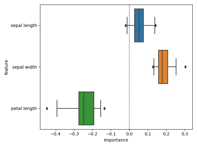
And check the differences in importances. We can now see that there is a difference in importances.
diff_fi = (
    cr_fi.set_index(["feature", "fold"])["importance"]
    - ncr_fi.set_index(["feature", "fold"])["importance"]
)
sns.boxplot(
    x="importance", y="feature", data=diff_fi.reset_index(), whis=[2.5, 97.5]
)
plt.axvline(0, color="k", ls=":")
plt.tight_layout()
Total running time of the script: (0 minutes 7.494 seconds)