Faces Decomposition

Implemented based on scikit-learn’s decomposition example.

Authors: Federico Raimondo, Vlad Niculae, Alexandre Gramfort

License: BSD 3 clause

from numpy.random import RandomState
import matplotlib.pyplot as plt
import seaborn as sns

from sklearn.datasets import fetch_olivetti_faces
from sklearn import decomposition

from opnmf import model, logging

Out:

/opt/hostedtoolcache/Python/3.8.12/x64/lib/python3.8/site-packages/seaborn/cm.py:1582: UserWarning: Trying to register the cmap 'rocket' which already exists.
  mpl_cm.register_cmap(_name, _cmap)
/opt/hostedtoolcache/Python/3.8.12/x64/lib/python3.8/site-packages/seaborn/cm.py:1583: UserWarning: Trying to register the cmap 'rocket_r' which already exists.
  mpl_cm.register_cmap(_name + "_r", _cmap_r)
/opt/hostedtoolcache/Python/3.8.12/x64/lib/python3.8/site-packages/seaborn/cm.py:1582: UserWarning: Trying to register the cmap 'mako' which already exists.
  mpl_cm.register_cmap(_name, _cmap)
/opt/hostedtoolcache/Python/3.8.12/x64/lib/python3.8/site-packages/seaborn/cm.py:1583: UserWarning: Trying to register the cmap 'mako_r' which already exists.
  mpl_cm.register_cmap(_name + "_r", _cmap_r)
/opt/hostedtoolcache/Python/3.8.12/x64/lib/python3.8/site-packages/seaborn/cm.py:1582: UserWarning: Trying to register the cmap 'icefire' which already exists.
  mpl_cm.register_cmap(_name, _cmap)
/opt/hostedtoolcache/Python/3.8.12/x64/lib/python3.8/site-packages/seaborn/cm.py:1583: UserWarning: Trying to register the cmap 'icefire_r' which already exists.
  mpl_cm.register_cmap(_name + "_r", _cmap_r)
/opt/hostedtoolcache/Python/3.8.12/x64/lib/python3.8/site-packages/seaborn/cm.py:1582: UserWarning: Trying to register the cmap 'vlag' which already exists.
  mpl_cm.register_cmap(_name, _cmap)
/opt/hostedtoolcache/Python/3.8.12/x64/lib/python3.8/site-packages/seaborn/cm.py:1583: UserWarning: Trying to register the cmap 'vlag_r' which already exists.
  mpl_cm.register_cmap(_name + "_r", _cmap_r)
/opt/hostedtoolcache/Python/3.8.12/x64/lib/python3.8/site-packages/seaborn/cm.py:1582: UserWarning: Trying to register the cmap 'flare' which already exists.
  mpl_cm.register_cmap(_name, _cmap)
/opt/hostedtoolcache/Python/3.8.12/x64/lib/python3.8/site-packages/seaborn/cm.py:1583: UserWarning: Trying to register the cmap 'flare_r' which already exists.
  mpl_cm.register_cmap(_name + "_r", _cmap_r)
/opt/hostedtoolcache/Python/3.8.12/x64/lib/python3.8/site-packages/seaborn/cm.py:1582: UserWarning: Trying to register the cmap 'crest' which already exists.
  mpl_cm.register_cmap(_name, _cmap)
/opt/hostedtoolcache/Python/3.8.12/x64/lib/python3.8/site-packages/seaborn/cm.py:1583: UserWarning: Trying to register the cmap 'crest_r' which already exists.
  mpl_cm.register_cmap(_name + "_r", _cmap_r)

set up logging

logging.configure_logging(level='INFO')

Out:

2021-11-09 12:43:59,308 - opnmf - INFO - ===== Lib Versions =====
2021-11-09 12:43:59,309 - opnmf - INFO - numpy: 1.19.5
2021-11-09 12:43:59,309 - opnmf - INFO - scipy: 1.7.2
2021-11-09 12:43:59,309 - opnmf - INFO - sklearn: 0.24.2
2021-11-09 12:43:59,309 - opnmf - INFO - opnmf: 0.0.2
2021-11-09 12:43:59,309 - opnmf - INFO - ========================

We will plot 6 faces and factorize to 6 components

n_row, n_col = 2, 3
n_components = n_row * n_col
image_shape = (64, 64)
rng = RandomState(0)

Load faces data

faces, _ = fetch_olivetti_faces(return_X_y=True, shuffle=True,
                                random_state=rng)
n_samples, n_features = faces.shape

print("Dataset consists of %d faces" % n_samples)

Out:

downloading Olivetti faces from https://ndownloader.figshare.com/files/5976027 to /home/runner/scikit_learn_data
Dataset consists of 400 faces

Defile plotting function

def plot_gallery(title, images, n_col=n_col, n_row=n_row, cmap=plt.cm.gray):
    plt.figure(figsize=(2. * n_col, 2.26 * n_row))
    plt.suptitle(title, size=11)
    for i, comp in enumerate(images):
        plt.subplot(n_row, n_col, i + 1)
        vmax = max(comp.max(), -comp.min())
        plt.imshow(comp.reshape(image_shape), cmap=cmap,
                   interpolation='nearest',
                   vmin=-vmax, vmax=vmax)
        plt.xticks(())
        plt.yticks(())
    plt.subplots_adjust(0.01, 0.05, 0.99, 0.93, 0.04, 0.)

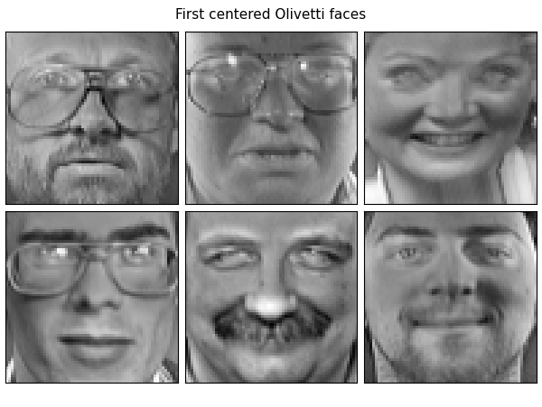
Let’s see how the first 6 faces look (centered around the mean) global centering

faces_centered = faces - faces.mean(axis=0)
# local centering
faces_centered -= faces_centered.mean(axis=1).reshape(n_samples, -1)
plot_gallery("First centered Olivetti faces", faces_centered[:n_components])

Lets set some parameters

init = 'nndsvd'
tolerance = 5e-3

NMF and OPNMF are both bi-factor factorization. The shared idea is that given a non-negative input matrix \(X \in \mathbb{R}^{m \times n}\), one tries to find two non-negative matrix \(W \in \mathbb{R}^{m \times r}\) and \(H \in \mathbb{R}^{r \times m}\) such that:

\[X \approx WH\]

In scikit-learn’s terminology, fit_transform will return \(W\) while \(H\) will be stored as the components_ attribute of the estimator.

estimator = decomposition.NMF(
    n_components=n_components, init=init, tol=tolerance)
W = estimator.fit_transform(faces)
H = estimator.components_

print(W.shape)
print(H.shape)

Out:

/opt/hostedtoolcache/Python/3.8.12/x64/lib/python3.8/site-packages/sklearn/decomposition/_nmf.py:1090: ConvergenceWarning: Maximum number of iterations 200 reached. Increase it to improve convergence.
  warnings.warn("Maximum number of iterations %d reached. Increase it to"
(400, 6)
(6, 4096)

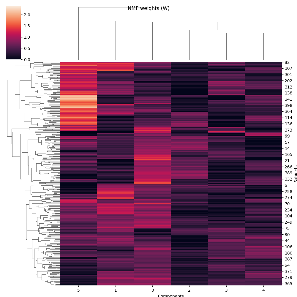
Now H (the components) is a 6 by 4096 matrix (n_components x pixels) and W (the weights) is a 400 by 6 matrix (n_samples x n_components) We can actually plot the components as images and the weights as a cluster map.

plot_gallery('NMF components (H)', H[:n_components])

g = sns.clustermap(W)
g.fig.suptitle('NMF weights (W)')
g.ax_heatmap.set_xlabel('Components')
g.ax_heatmap.set_ylabel('Subjects')

• 
• 

Out:

Text(990.5555555555553, 0.5, 'Subjects')

Contrary to NMF, Projected Non-Negative Matrix Factorization (PNF), is defined such that:

\[X \approx PX\]

where \(P = WW^{T}\).

This expands to:

\[X \approx WW^{T}X\]

In consecuence \(H=W^{T}X\)

The Orthonormal Projected Non-Negative Matrix Factorization (OPNMF), adds another constraint to \(W\): orthonormality.

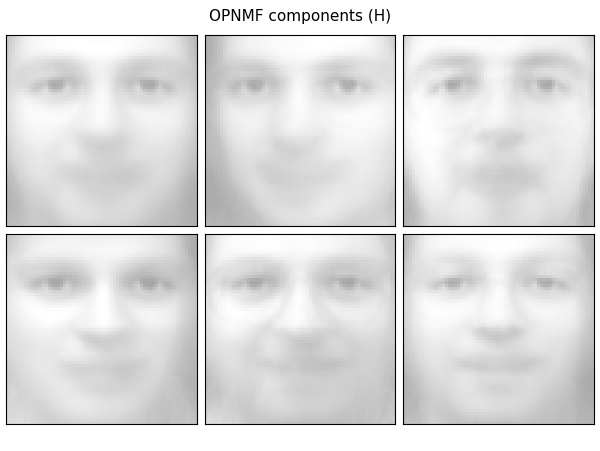
Let’s do the same figures as with NMF

estimator = model.OPNMF(n_components=n_components, init=init, tol=tolerance)
W = estimator.fit_transform(faces)
H = estimator.components_
plot_gallery('OPNMF components (H)', H[:n_components])

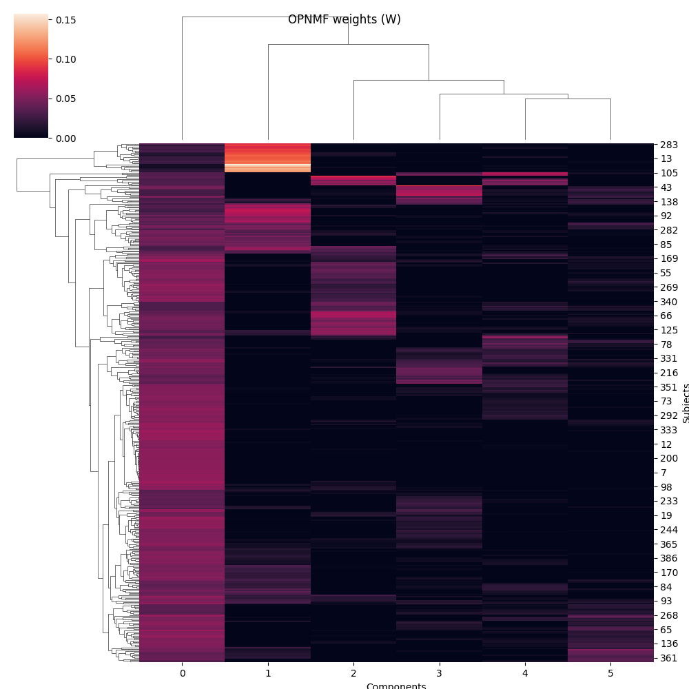
g = sns.clustermap(W)
g.fig.suptitle('OPNMF weights (W)')
g.ax_heatmap.set_xlabel('Components')
g.ax_heatmap.set_ylabel('Subjects')

• 
• 

Out:

2021-11-09 12:44:02,069 - opnmf - INFO - Initializing using nndsvd
2021-11-09 12:44:02,127 - opnmf - INFO - iter=0 diff=0.9636635184288025, obj=155.62832641601562
2021-11-09 12:44:02,157 - opnmf - INFO - Converged in 80 iterations

Text(990.5555555555555, 0.5, 'Subjects')

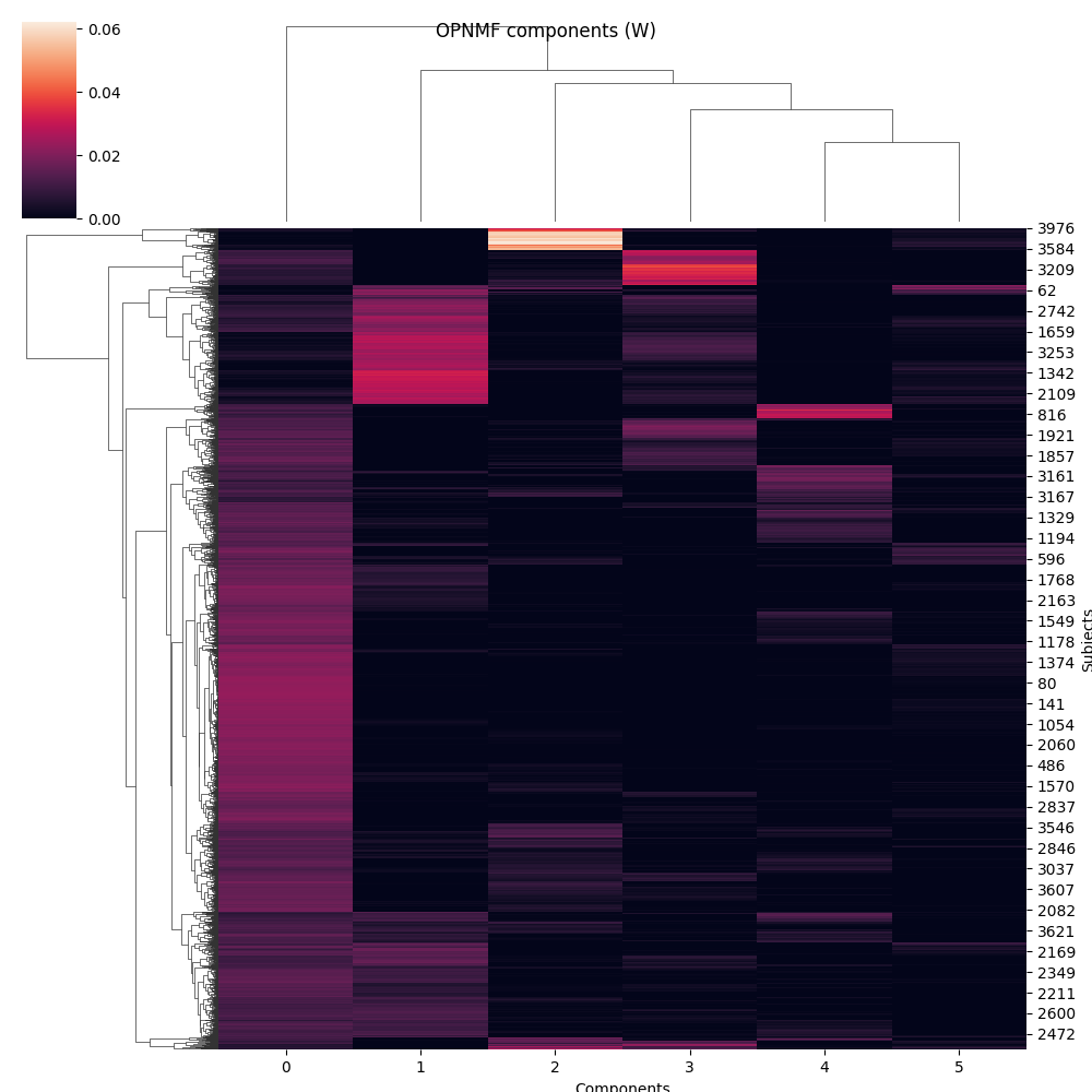
From these plots, we can see that OPNMF seems to do some sort of clustering over the first dimension of X. As the orthonormality constraint forces every subject to have a positive weight with at most one component, it defines components in a way that each subject matches only one.

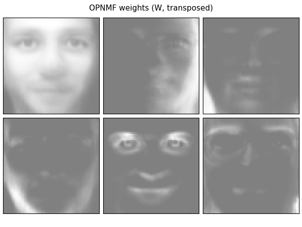
Interestingly, we can use this methodology to do so on the other dimension (pixels in the image)

estimator = model.OPNMF(n_components=n_components, init=init, tol=tolerance)
W = estimator.fit_transform(faces.T)  # Transpose the faces
H = estimator.components_

print(W.shape)
print(H.shape)

Out:

2021-11-09 12:44:02,872 - opnmf - INFO - Initializing using nndsvd
2021-11-09 12:44:03,164 - opnmf - INFO - iter=0 diff=0.9637103080749512, obj=155.67025756835938
2021-11-09 12:44:06,361 - opnmf - INFO - iter=100 diff=0.00534751545637846, obj=146.4695281982422
2021-11-09 12:44:06,814 - opnmf - INFO - Converged in 114 iterations
(4096, 6)
(6, 400)

In this case, H (the components) is a 6 by 400 matrix (n_components x n_samples) and W (the weights) is a 4096 by 6 matrix (pixels x n_components). So now we can plot W as images and H as a cluster map.

plot_gallery('OPNMF weights (W, transposed)', W[:, :n_components].T)

g = sns.clustermap(W)
g.fig.suptitle('OPNMF components (W)')
g.ax_heatmap.set_xlabel('Components')
g.ax_heatmap.set_ylabel('Subjects')

• 
• 

Out:

/opt/hostedtoolcache/Python/3.8.12/x64/lib/python3.8/site-packages/seaborn/matrix.py:654: UserWarning: Clustering large matrix with scipy. Installing `fastcluster` may give better performance.
  warnings.warn(msg)

Text(990.5555555555555, 0.5, 'Subjects')

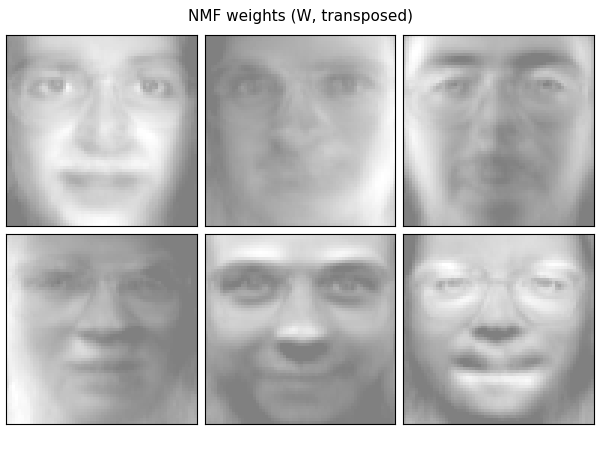
We can also do the same with NMF, but there will be no effect. Assuming \(X^T=\tilde{X}\) and the following NMF:

\[\tilde{X} \approx \tilde{W}\tilde{H}\]

Then the solution \(X \approx WH\) can be also used:

\[\tilde{X} = X^T \approx (WH)^T\]

which expands to:

\[\tilde{X} = X^T \approx H^TW^T\]

So from the first formula: \(\tilde{W}=H^T\) and \(\tilde{H}=W^T\)

estimator = decomposition.NMF(
    n_components=n_components, init=init, tol=tolerance)
W = estimator.fit_transform(faces.T)  # Transpose the faces
H = estimator.components_

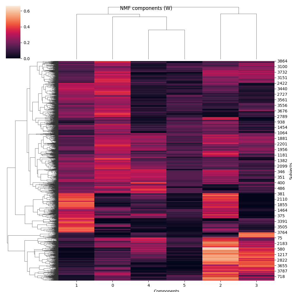
plot_gallery('NMF weights (W, transposed)', W[:, :n_components].T)

g = sns.clustermap(W)
g.fig.suptitle('NMF components (W)')
g.ax_heatmap.set_xlabel('Components')
g.ax_heatmap.set_ylabel('Subjects')

• 
• 

Out:

/opt/hostedtoolcache/Python/3.8.12/x64/lib/python3.8/site-packages/sklearn/decomposition/_nmf.py:1090: ConvergenceWarning: Maximum number of iterations 200 reached. Increase it to improve convergence.
  warnings.warn("Maximum number of iterations %d reached. Increase it to"
/opt/hostedtoolcache/Python/3.8.12/x64/lib/python3.8/site-packages/seaborn/matrix.py:654: UserWarning: Clustering large matrix with scipy. Installing `fastcluster` may give better performance.
  warnings.warn(msg)

Text(990.5555555555555, 0.5, 'Subjects')

If you want to follow the original explanaition with much more math, see:

Z. Yang and E. Oja, “Linear and Nonlinear Projective Nonnegative Matrix Factorization,” in IEEE Transactions on Neural Networks, vol. 21, no. 5, pp. 734-749, May 2010, doi: 10.1109/TNN.2010.2041361.

plt.show()